So tell me what it means.

We are standing in the hallway outside Track 2. My colleague has gotten awkawardly silent. I had asked a simple probability question.

You mean, like its actual defintion?

Tell what it means. Tell what is the definition of a random variable.

He is looking around, he is looking up the glass ceiling many feet in the air. The answer he was looking for wasn’t up there. Hopefully, the clouds clear his mind.

It’s a quantity that can take on multiple values based on probability distribution.

That’s not it

---

Some episode like this has happened over and over again for the last year or so, and it always goes down roughly the same way. Why is this going on?

Random Variables are usually very poorly explained. Once you get past the deceptive name, you have unintuitive notation that hides and obscures what is actually going on. In the following post, I will first explain what are random variables. Then define probability, conditional probabity, expectation and variance in terms of them.

Probability Spaces

First, let’s define some things, namely probaility. In the modern formulation probailities are measures in a probability space. By this, we mean a model with these three things.

\(\large (\Omega, E, P)\)

\(\Omega\) is the sample space. It is the set of world states. These are sometimes called outcomes. If we were gambling, this is possible ways a game could end.

\(E\) is the event space. It is the set of subsets of \(\Omega\). If we were gambling. Each element of \(E\) is something we could place a bet on.

\(P\) is the probaility measure. This is a function that for each element of \(E\) assigns a probability between 0 and 1.

As a basic example, consider a six-sided die:

The sample space is {1,2,3,4,5,6}. The event space is every subset of that space. Some elements of the event space include {}, {1,3,5}, and {4}. These correspond to betting on none of the outcomes (a bet you will surely lose), betting on an odd number, and betting on the number 4. Assuming all these outcomes are equally likely.

\[ P(\left\{\right\}) = 0 \] \[ P(\left\{1,3,5\right\}) = \frac{1}{2} \] \[ P(\left\{3\right\}) = \frac{1}{6} \]

The trouble with this formulation is its cumbersome to work within directly. Random variables provide a way to summarize the quantities we want to find the probabilities of in terms of samples.

Enough burying the lead. What are random variables?

Random Variables are functions from samples to real numbers/vectors

\(\large X : \Omega \rightarrow \mathbb{R^n}\)

That’s it. Nothing complicated or fancy. This is the definition in nearly any probability or statistics book I have opened. If your book does not have a definition that is essentially the above, burn it. Remember its not a number, its a function.

Random variables exist as a necessary abstraction over probability spaces and allow us to reason about sets of events in a clean way.

Here is an example random variable:

\[ Odd(\omega) = \cases{ 1 & \text{if } \omega \text{ is odd} \cr 0 & \text{if } \omega \text{ is even} } \]

Random variables implicitly transform a given probability space into a related one where the range of the function defines the new sample space. Since, the range defines a new space, we can compose these functions to produce arbitrary distributions.

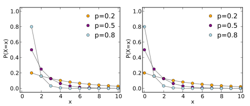
We can define a function to access these probabilities. If our random variable is discrete this is called the probability mass function.

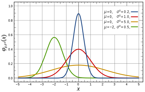
If our random variable is continuous then this will be referred to as a probability density function. The thing to note with this curve, probabilities aren’t the values on the y-axis, they are they areas under the curve.

For our example random variable the equation becomes:

\(\large \mathbb{P}[Odd = 1] := P(\{\omega \in \Omega : Odd(\omega) = 1\})\)

Notice those Ps aren’t the same. The left one is the probability mass function. The right one is probability measure from before. In the standard notation X refers to a random variable. x refers to the value it will return.

When you see P[X], P(X), p(x), or P(X = x) these are probability mass functions. In fact, only P(X = x) even defines a probability. The others are parameterized functions since we don’t know for which value of X do we want the probability. This is why the probability mass function is sometimes written \(f_X(x)\) .

Note: in practice we don’t define probability density functions in terms of a sample space. We usually just say the range of random variable comes from one of a standard prefined distributions.

Joint and Conditional Probability

Usually though we will have more than one random variable and they will have different things to same about a probability space.

The joint probability is probability space defined by the cartesian product of two random variables. It is defined as

\[ \large \mathbb{P}(X = x, Y = y) = P(\{\omega \in \Omega : X(\omega) = x \cap Y(\omega) = y \}) \]

This can be informally thought of as the probability X = x and Y = y.

The conditional probability can be thought of asking what is probability X = x assuming we know Y = y. To use our running example, assuming we knew the die was odd what’s the chance it landed 3.

Conditional probability is defined

\[ \large \mathbb{P}(X = x | Y = y) = \frac{\mathbb{P}(X = x, Y =y)}{\mathbb{P}(Y = y)} \]

This is sometimes called the Chain Rule. Specifically this is phrased as:

\[ P(X, Y) = P(Y)P(X | Y) \]

Many times you will see x and y dropped from these definitions. This implies these equations for all values of x and y.

Expectation

Expectation are the important quantity. Whenever you are discussing the quantities you wish to use probability theory for, the quantities in question will be expectations. Do I expect to make money if I keep playing at this poker table? How much can I expect to lose playing the lottery? How many voters do we expect to vote this election? How many students are expected to pass the class? All these quantities are what is actually cared about. Probabilities are just numbers for weighting the different events. Expectation are one the quantities we learn that really summarize what a distribution is saying.

\[ \large \mathbb{E} [X] = \large \int x p(x) dx \]

Interestingly, its debatable whether probabilities or expectations are more fundamental. We can describe probabilities are just expectations over indicator functions that return 1 for a desired event and 0 otherwise. This also means, that you do want the probability of an event, who should still take the expectation of the indicator function representing that event.

Conditional Expectation

Interestly, we can also take expectations over conditional probability distributions. This is because a conditional distribution is like a distribution.

\[ \large \mathbb{E} [X | Y = y] = \large \int x p(x | y) dx \]

Law of the Lazy Statistician

A large degree of the power of random variables actually comes from a theorem that is used so frequently it never gets mentioned. This theorem is called the Law of the Lazy Statistician. It can essentially stated as follows:

\[ \large \mathbb{E} [g(X)] = \large \int g(x)p(x) dx \]

This is amazing, because we can take expectations over arbitrary functions on the random variable. Even more amazing is we never need to explicit represent the new probability space denoted by the range of g. We can directly work in the probability distribution associated with X. This is handy, because this new probability distribution can easily be nothing like the base distribution.

The proof of this is fairly straightfoward. We rearrange the sum to count each possible value of y for g(X)

\[ \large \int g(x) p(x) dx = \large \int y \int_{\{ x : g(x) = y \}} p(x) dx dy \]

This inner term is equivalent to the probability of each y value

\[ \large \int g(x) p(x) dx = \large \int y p(y) dy \]

Which is the definition of expectation in Y with \(Y = g(X)\)

Variance

As an example, we will use this theorem to calculate the variance of a random variable.

\[ \large Var(X) = \large \mathbb{E}[(X - E[X])^2] \]

Now the inner expectation can simply be evaluated for X and give the result \(\mu\). At this point we are taking the expectation of an implicit function Y

\[ \large Y(\omega) = \large (\omega - \mu)^2 \]

And thanks to the law of the lazy statistician, we can use the probability mass function of X instead of having to explicitly find the probabilities for each of values of Y. Not having to do that work, means we can define a probability function that is easy to work, and then stack random variables to compute the quantities we actually care about.

Conclusions

There are large parts of probability and statistics I haven’t covered. Random Variables are at the core of both fields, so if you do analytics, you really ought to know the definition.